Challenge:� The Case for a Strong $US?
�World opinion has overwhelmingly supported the notion that the �fundamentals� point to a �dangerously over valued� $US.� These include the �record� trade gap, �record� budget deficit, increased energy costs, a sluggish domestic economy, and eroding �confidence� in the $US.� This confluence has been deemed �unsustainable� and for all practical purposes �correctible� only by a further fall in the $US.� However, while these are perhaps true observations, with a closer look in a broader context the $US begins to look undervalued, and could be poised for a substantial rally.
�The factors that mainstream and popular analysis associate with currency valuation include interest rate differentials, current account deficits, GDP differentials, govt. budget deficits, and intangibles such as �confidence.�� Unfortunately, most of these are not reliable indicators.� Japan, for example, has had 7% budget deficits, a 0% interest rate policy, weak GDP growth, and low levels of confidence, as well as little or no international yen savings, yet the yen has been very strong for a number of years.� The one positive is Japan�s current account surplus, yet the $Australia, for example, has been strong even though Australia has a current account deficit, so that alone can�t be the dominant variable.� I�ll next look at these variables on an individual basis.
�The current account deficit is a function of the non resident (�rest of the world�) desire to net save financial assets of that currency.� If this savings desire is sufficiently strong and growing there can be a large and growing current account deficit without currency depreciation and without rising import prices.� The reverse is also the case.� If the non resident savings desire is falling the evidence can be a depreciating currency and possibly higher import prices.
�The problem is quantifying this savings desire.� It can be purely political, as when the BOJ (Bank of Japan) buys $US.� It can also be institutional, as when a government establishes superannuation rules, or when a world �model portfolio� is established and promoted.
�Currency fluctuations can also be functions of short term and intermediate term shifts.� For example, if a large holder of $US reserves decides to diversify them over a 3 year period, currency values could be affected for the entire 3 years.�
�Recognizing that by identity a govt. budget deficit (surplus) = non govt surplus (deficit) all in terms of net financial assets of that currency, it follows that for a given non resident savings desire (assuming domestic savings desires are constant) undiscounted changes in the fiscal balance will alter the level of the currency.� (Note that this is the �quantity theory� identity in it�s �purest� form.)�
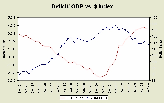
�The following graph shows the $US index verses the seasonally adjusted quarterly US budget deficit as a % of GDP.� Recall that there was a spike in Q3, 2003 was due to the retroactive portion of the tax cuts, which was instrumental in creating a bulge in $US financial assets that overcame existing savings desires, thereby contributing to the falling $US.� In the latest quarter, however, the US budget deficit has fallen considerably further, and while the graph is showing year over year changes, the US deficit may currently be annualizing at only 3% of GDP.� This is less than the Eurozone�s and less than half of Japan�s budget deficits as %s of GDP.� It is not unreasonable to expect the dollar to regain lost ground, and appreciate towards previous levels, as it reacts to this �external shock� to the balance between non resident savings desires and total savings available.
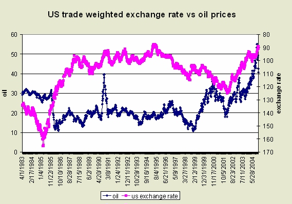
Likewise, an unanticipated change in the price of imported oil may function as a �supply shock� to available savings for non residents.� For example, an increase in the $US price of oil may cause net $US expenditures on imports to rise, thereby driving an increase in non resident savings (and a decrease in resident savings) that could lower the value of the $US.� Note the graph of the $US index versus the price of crude (recognizing the graph doesn�t show causation):
�
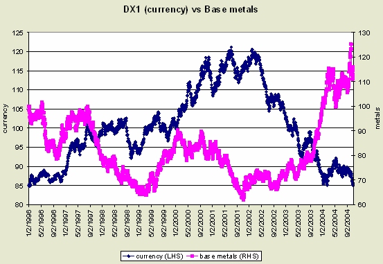
In addition to energy, metals also may have peaked, as higher prices brought out more supply from higher cost producers.� In previous commodity cycles, prices rose until excess supply was brought to the market, and we may be at or near that point in the current cycle.
There is a further complexity at work, as the countercyclical tax code interacts with economic growth.� The story goes like this, and it�s a relatively new story:� It begins with unemployment high enough to be able to fall substantially.� As a recovery begins (either because of rising export demand or, more commonly, rising domestic demand do to a sufficiently large govt. budget deficit), the newly employed immediately buy cars, etc. on credit.� So a new income of perhaps $700 per week results in borrowing to spend perhaps $15,000, often as a necessary expenditure to get to work.� Rather than a �multiplier� effect this is an �accelerator� effect.� It also lowers the govt. deficit as the countercyclical income tax kicks in.� As a consequence of this accelerating increase in demand GDP increases and domestic savings declines (debt increases, govt. deficit falls) and therefore financial leverage increases both by the increasing consumer debt and suppression of domestic net financial assets due to the �improving� fiscal balance.� And, of course, employment increases, thereby sustaining this accelerating growth/accelerating leverage combination.� This process is typically correlated to a strong currency as well, along with rising consumer imports.� Look to Japan in the late 80�s, the US in the late 90�s and Australia and the UK in the last few years as examples.� Japan has probably not yet entered that stage, but may be getting close after several years of financial equity and demand replenishing deficits.� This phase necessarily ends when gains in employment slow as the pool of unemployed decreases, and/or the domestic �financial burdens ratio� increases towards the limits of debt service and other payments relative to income.� This is followed by a period of slack demand, as domestic debt can no longer grow sufficiently to sustain employment, and net financial assets are seriously deficient due to the fiscal balance.� Without a proactive shift in fiscal balance towards sufficient deficits to sustain demand, the deficit grows instead via deficient revenues due to the demand deficient economic weakness.� The transition from the accelerator phase to the slack demand phase is often described as �bursting of the bubble� or �hitting the wall.�
Nations in this accelerator phase have experienced relatively strong currencies.� I would credit this to the tightening fiscal positions due to counter cyclical tax structures, combined with a rising non resident demand for financial assets of that currency, as this phase is also attracting foreign investment, both direct and portfolio.� After �hitting the wall� this process is reversed, as the rising budget deficit due to economic weakness and the reduced non resident savings desires due to the relative lack of attractive investments combine to weaken the currency.
Japan, however, will be faced with a different type of expansion.� The context will be relatively weak external demand which may dampen exports, with domestic demand accelerating, driving an accelerating demand for consumer imports.
The Bank of Japan has not intervened since March 04, and the $/yen has held at levels above the point of BOJ intervention for almost 9 months.� This indicates the trade flows are no longer causing a deficiency of yen outside of Japan.
The strong $ and falling import prices, particularly energy, in the context of relatively weak domestic demand and a substantial output gap can quickly resurrect the spectre of US deflation.� Meanwhile, however, the Fed is raising rates do to a misguided notion of �real interest rates� and their relation to the macro economy.� For nearly 30 years the Fed was guided by a theory that concluded lower unemployment would result in higher �inflation,� but this was unceremoniously abandoned after 2,000 when unemployment dipped below 4% and core CPI continued lower.� This theory was just as unceremoniously replaced by an even older (fixed exchange rate!) theory that �neutral� monetary policy means the nominal rate be set at some spread over �inflation,� and that �accomodative� monetary policy resulted from the nominal rate being set at some rate below �inflation.�� Therefore, with core CPI around 1.5%-2%, we can expect the Fed not to �feel comfortable� until they raise the fed funds rate to about 3.5%.� And only with very obvious economic weakness is it likely the Fed will reverse course and become �accomodative� with lower �real� rates.
Warren Mosler
Jan 4, 2004
Note:� This was first written two weeks ago, and the charts do not include this weeks market action.� The $ has strengthened, West Texas Crude remains below $44 per barrel, and the Fed minutes show a determination to continue to raise rates.
Posted 1/5/2005